🐿️ 1.8 Object Detection

To make robots see, we need to create a way for them to interpret the world. One solution is object detection: drawing boxes around objects we want a computer to identify in an image.

Introduction

What is YOLO?

While many associate the term "YOLO" with “You Only Live Once,” the computer vision term is actually a lot cooler:

You Only Look Once.

This play on words is meant to demonstrate one of YOLO’s most important features. Instead of traditional two-stage methods, which first scan the image to propose regions and then go back to classify them, yolo does this all in one sweep.

For example, models like Faster R-CNN first generate possible object regions, then classify each proposed region. YOLO does both localization and classification in a single forward pass through the network.

Yolo works by splitting an image into an S x S grid. Each cell is responsible for detecting objects whose center point is in that cell.

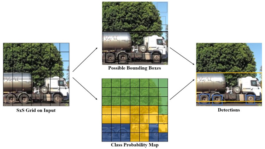
YOLO Detection Sequence. Source: Marcomini, L., & Cunha, A. L. (2022). Truck Axle Detection with Convolutional Neural Networks. Used under CC BY-NC-SA 4.0.

The detector takes part in three main modules:

1. Backbone - extracts useful features from an image, similar to the CNN you made earlier.
2. Neck - refines these extracted features.
3. Head - predicts the bounding boxes, classes, and confidence scores.

Why is YOLO a good model for AUVs?

Yolo by itself is fast. This makes it useful for AUVs, since these robots must be able to process inputs quickly to make decisions.

Coupled with external packages like ncnn and OpenCV, yolo is the perfect model to guide your AUV.

Dataset Annotation

You have your data. Now it is time for annotation.

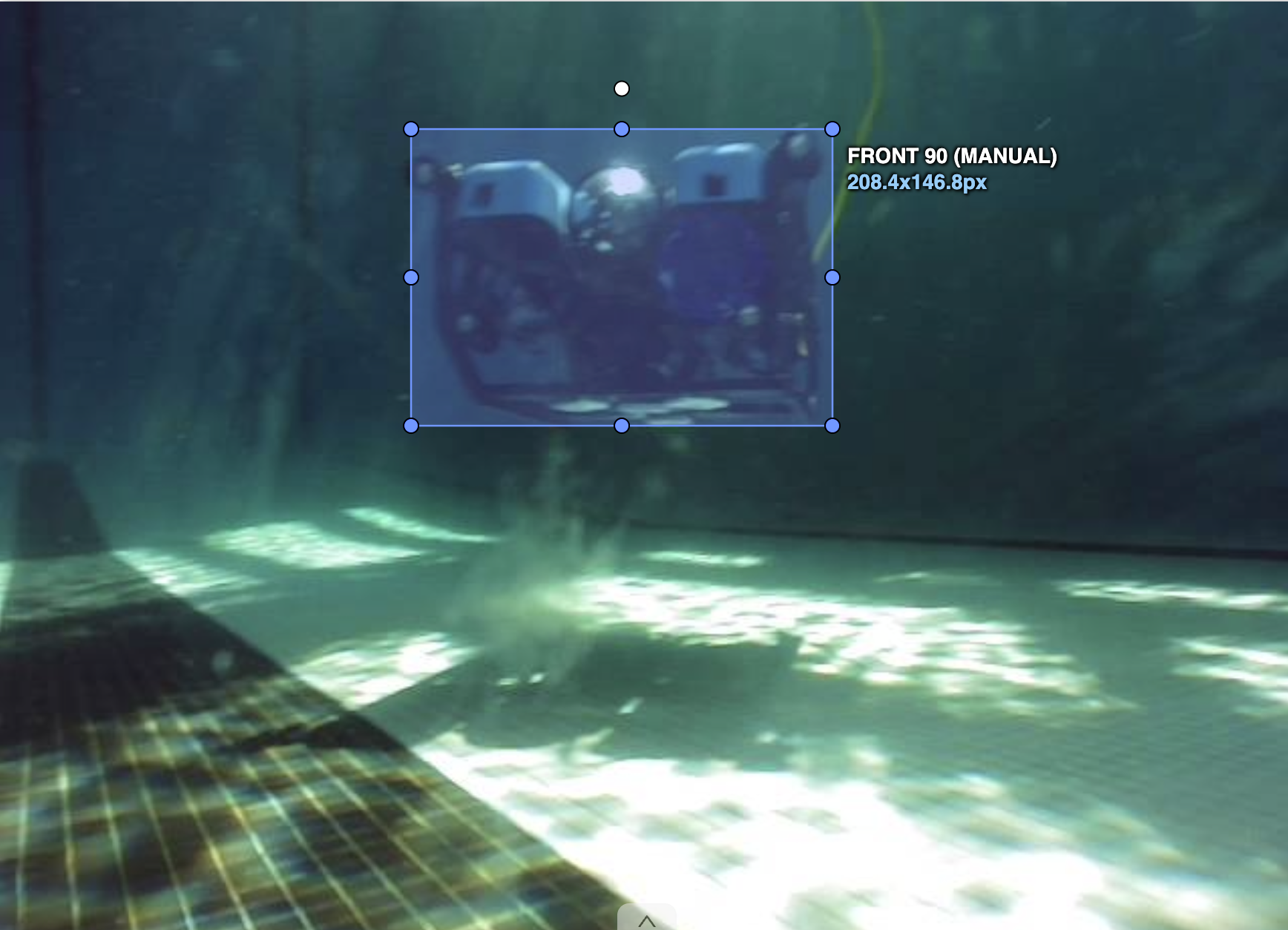
Yolo trains on examples of bounding boxes, or boxes around your object, to learn to detect. That means that every single image in your dataset needs to be labelled.

Roboflow

Roboflow is an online computer vision platform. On it, you can:

• Annotate Data
• Train Models
• Preprocess Datasets
• Work with Teams

We will be using Roboflow for the data annotation and preprocessing. For training, we will be using Ultralytics, a package that provides many pre-trained versions of YOLO.

Open Roboflow and create a new account:

https://roboflow.com/annotate

If you are uploading the data for your group, create a new workspace. Select the public plan. When it asks you to invite your team, invite your teammates or create a public link. Then select Use my own data.

Create a new project. Give it a title, select Object Detection, and then select Use Traditional Model Builder Instead.

When you get access to the project page, upload your dataset using the Select Folder button. Then click Save and Continue.

After the data is uploaded, select Label with my team and choose your (willing) team members.

Labeling Images

To label your data, select the dataset in the Annotations tab.

Click Start Annotating.

Select the bounding box tool in the toolbar on the right, or use the hotkey B.

Drag a bounding box over your subject of interest. Make sure the box edges touch the edges of the object as closely as possible.

After you finish drawing a bounding box, you will get the option to create a new class.

A class is the type of object you want your model to identify. For instance:

• Single-class Detection: just “Squirrel” or nothing
• Multi-class Detection: “Squirrel” “Bunny” “Fish” “Rat”

Name your class.

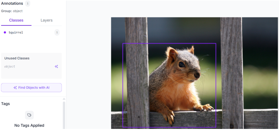
Once you are done annotating the image, click the checkmark at the top to add the image and annotation to your dataset, which will make the next image automatically pop up. You do not need to press the next button.

Happy labeling!

Dataset Splits

After you finish labeling, go to the Versions tab.

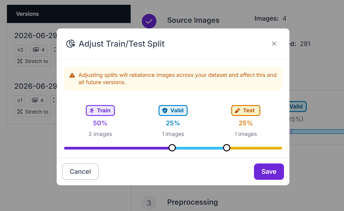
Here, you will create the train, validation, and test splits.

We split the dataset so that we have:

• Training data - Data that will be used to actually teach the model.
• Validation data - Data that the model has never seen before in training. Val is used to validate that our model is improving during training, generally assessed after every epoch. This improvement metric is necessary for systems such as Early Stopping (stopping training after metrics seem to plateau) and Learning Rate schedulers.
• Testing data - Also data that has never been seen by the model, neither in training or for lr schedulers/early stop. Testing data is vital for identifying the true model performance. These are the final metrics that should be reported.

While these values are largely up to you, a good starting point is:

• 75% training
• 10% validation
• 15% testing

Click Rebalance and drag the knobs to change the percentages.

Preprocessing

For the next step, preprocessing, explore the various preprocessing steps Roboflow gives you. Consider how each can have an effect on the processing power required to run YOLO locally.

For now, set resize to:

512 x 512

Then continue.

Skip augmentation for now.

Click Create, then Download Dataset.

Export the dataset in YOLO26 format as a ZIP file.

Unzip the file and explore the following:

• data.yaml
• images/
• labels/

Try to predict what each file or folder is for, and how the label files are structured.

Check-Off

• Create a Roboflow account.
• Upload your dataset.
• Annotate at least a few images.
• Create train, validation, and test splits.
• Export the dataset in YOLO format.
• Open the data.yaml file and inspect it.
• Open a label .txt file and try to understand its format.

Training

Model

We will be using YOLO v26n (nano) with the Ultralytics package. Nano models are small and fast, which makes them good for running on Raspberry PIs.

Google Colab Set-up

We will be training on Google Colab T4 GPUs. They’re free and much faster to use than normal CPUs.

To set up, go to Google Colab and make a new notebook.

Select the dropdown next to Connect in the top right and choose Change runtime type.

Set the hardware accelerator to:

T4 GPU

Then save and connect to the runtime.

Install Requirements

Run this in a Colab cell:

!pip install ultralytics opencv-python numpy matplotlib Pillow

Mount Google Drive

To use your data, upload your unzipped dataset folder to your Google Drive.

In Colab, go to:

Files -> Folder button -> Mount Drive

Import Dependencies

import os
import matplotlib.pyplot as plt
from ultralytics import YOLO
from PIL import Image
import cv2
import numpy as np

Reading the Dataset

First, set the path to your dataset.

path_to_dataset = "/content/drive/MyDrive/<path_to_your_dataset_here>"

Your dataset should look something like this:

yolo_dataset/
├── data.yaml
├── train/
│   ├── images/
│   └── labels/
├── valid/
│   ├── images/
│   └── labels/
└── test/
    ├── images/
    └── labels/

Use os.listdir to inspect the image and label files:

image_files = os.listdir(path_to_dataset + "/train/images/")
print(image_files)

label_files = os.listdir(path_to_dataset + "/train/labels/")
print(label_files)

Displaying Images

To display images, use Image from the PIL library (pillow) and plt from matplotlib.pyplot.

image_files_view = image_files[:4]
path_to_images = path_to_dataset + "/train/images/"

fig, axes = plt.subplots(1, 4, figsize=(15, 5))

for i, filename in enumerate(image_files_view):
    full_path = os.path.join(path_to_images, filename)
    img = Image.open(full_path)
    axes[i].imshow(img)
    axes[i].set_title(filename, fontsize=10)
    axes[i].axis("off")

plt.tight_layout()
plt.show()

Understanding YOLO Labels

YOLO label files are stored as .txt files.

Each line in a label file represents one bounding box:

class_id center_x center_y width height

The important part is that YOLO coordinates are normalized, meaning that the numbers are between 0 and 1, not actual pixel values.

For example:

0 0.670 0.421 0.115 0.348

This means:

• 0 is the class ID.
• 0.670 is the normalized x-coordinate of the box center.
• 0.421 is the normalized y-coordinate of the box center.
• 0.115 is the normalized box width.
• 0.348 is the normalized box height.

Why does YOLO use normalized coordinates? Think about it. If the image is resized, the labels will still work, since it's always just a percentage.

Pairing Images and Labels

Pairing is very important in machine learning.

If your images and labels are mismatched, your model will attempt to learn gibberish.

path_to_images = path_to_dataset + "/train/images/"
path_to_labels = path_to_dataset + "/train/labels/"

pairs = []

for img in image_files:
    img_name = os.path.splitext(img)[0]

    for label in label_files:
        label_name = os.path.splitext(label)[0]

        if img_name == label_name:
            pairs.append((img, label))

print(pairs)

Displaying Bounding Box Overlays

Now let’s display images with their bounding boxes drawn on top.

fig, axes = plt.subplots(1, 4, figsize=(15, 5))

for i, pair in enumerate(pairs[:4]):
    img_filename, label_filename = pair

    img_path = os.path.join(path_to_images, img_filename)
    label_path = os.path.join(path_to_labels, label_filename)

    img = Image.open(img_path)
    width, height = img.size

    axes[i].imshow(img)
    axes[i].set_title(img_filename, fontsize=10)
    axes[i].axis("off")

    with open(label_path) as f:
        for line in f:
            print("bbox: " + line)

            parts = line.split()
            class_num = int(parts[0])
            center_x = float(parts[1])
            center_y = float(parts[2])
            b_width = float(parts[3])
            b_height = float(parts[4])

            # Convert YOLO coordinates to pixel coordinates.
            # YOLO coordinates are required by the model.
            # Pixel coordinates are required for visualization.
            x1 = (center_x - b_width / 2) * width
            y1 = (center_y - b_height / 2) * height
            box_w = b_width * width
            box_h = b_height * height

            rect = plt.Rectangle(
                (x1, y1),
                box_w,
                box_h,
                linewidth=1.5,
                edgecolor="red",
                facecolor="none",
            )

            axes[i].add_patch(rect)
            axes[i].text(
                x1,
                y1 - 4,
                str(class_num),
                color="red",
                fontsize=7,
                fontweight="bold",
            )

plt.tight_layout()
plt.show()

Check-Off

• Display four raw training images.
• Pair each image with its matching label file.
• Open a label file and print its bounding box values.
• Convert YOLO coordinates into pixel coordinates.
• Draw bounding boxes on top of the images.

Training YOLO

The Ultralytics package automatically recognizes valid YOLO dataset files when given a correct data.yaml file.

yaml_file = path_to_dataset + "/data.yaml"

MODEL = "yolo26n.pt"

model = YOLO(MODEL)
model.train(data=str(yaml_file), epochs=50, imgsz=640)
model.val(data=str(yaml_file))

After training, go into:

runs -> detect -> train

Here you will find metrics, results, and visual examples from the testing set.

Some useful files include:

• confusion_matrix.png
• results.png
• val_batch_pred.jpg
• val_batch_labels.jpg

Inference on a Custom Image

Finally, you can run inference on a custom image.

This means using your trained model to predict on new images, similarly how you will be using it with your AUV (if you do choose to use YOLO).

custom_image_path = "/content/drive/MyDrive/test.jpg"

model = YOLO("runs/detect/train/weights/best.pt")
results = model.predict(source=custom_image_path, save=True, conf=0.25)

The predictions will be saved automatically inside the runs/detect/predict folder.

You can also extract the bounding box information like so:

for box in results[0].boxes:
    x1, y1, x2, y2 = box.xyxy[0].cpu().numpy()
    print(f"Coordinates: ({x1}, {y1}), ({x2}, {y2})")
    class_num = int(box.cls[0].cpu().numpy())
    print(f"Class: {class_num}")
    confidence = float(box.conf[0].cpu().numpy())
    print(f"Confidence: {confidence}")

note

YOLO predicts outputs in pixel positions, not the normalized coordinates.

Problem Set

Problem 1: Run on RPI

Get your model to run locally on your RPI.

To install Ultralytics, ensure you only use the necessary packages.

1. Download your trained YOLO model from Colab. Files -> Right click on best.pt -> Download
2. Host your model files and an example image on GitHub. Make a new repo -> Upload best.pt -> Upload a squirrel test image
3. On the RPI, create a new virtual environment for object detection (make sure you are in your user):

mkvirtualenv object-detection
workon object-detection

4. Clone your repo.

git clone <repo link>

5. Inside the virtual environment, run the following commands:

pip install torch torchvision --index-url https://download.pytorch.org/whl/cpu
pip install ultralytics --no-deps
pip install opencv-python-headless pillow pyyaml requests tqdm psutil numpy matplotlib nvidia-ml-py opencv-python polars ultralytics-thop

6. Create a new python script to run YOLO.
7. Get your YOLO model to predict on your testing image.

info

When running YOLO on a continuous video stream using an RPI, it is important to optimize the model for performance. Consider looking into the ncnn library in the near future.